Καμπυλόγραμμη Συντεταγμένη

Καμπυλόγραμμον Σύστημα Συντεταγμένων

Curvilinear coordinates

Καμπυλόγραμμες Συντεταγμένες

Καμπυλόγραμμες Συντεταγμένες

Καμπυλόγραμμες Συντεταγμένες

Καμπυλόγραμμες Συντεταγμένες

Καμπυλόγραμμες Συντεταγμένες

Καμπυλόγραμμες Συντεταγμένες

Καμπυλόγραμμες Συντεταγμένες

Καμπυλόγραμμες Συντεταγμένες

Καμπυλόγραμμες Συντεταγμένες

Είναι ένα Σύστημα Συντεταγμένων.

Ετυμολογία

Η ονομασία "Καμπυλόγραμμη" σχετίζεται ετυμολογικά με την λέξη "καμπύλη".

Εισαγωγή

In geometry, curvilinear coordinates are a coordinate system for Euclidean space in which the coordinate lines may be curved. These coordinates may be derived from a set of Cartesian coordinates by using a transformation that is locally invertible (a one-to-one map) at each point. This means that one can convert a point given in a Cartesian coordinate system to its curvilinear coordinates and back. The name curvilinear coordinates, coined by the French mathematician Lamé, derives from the fact that the coordinate surfaces of the curvilinear systems are curved.

Well-known examples of curvilinear coordinate systems in three-dimensional Euclidean space (R³) are Cartesian, cylindrical and spherical polar coordinates. A Cartesian coordinate surface in this space is a plane; for example z = 0 defines the x-y plane. In the same space, the coordinate surface r = 1 in spherical polar coordinates is the surface of a unit sphere, which is curved. The formalism of curvilinear coordinates provides a unified and general description of the standard coordinate systems.

Curvilinear coordinates are often used to define the location or distribution of physical quantities which may be, for example, scalars, vectors, or tensors. Mathematical expressions involving these quantities in vector calculus and tensor analysis (such as the gradient, divergence, curl, and Laplacian) can be transformed from one coordinate system to another, according to transformation rules for scalars, vectors, and tensors. Such expressions then become valid for any curvilinear coordinate system.

Depending on the application, a curvilinear coordinate system may be simpler to use than the Cartesian coordinate system. For instance, a physical problem with spherical symmetry defined in R³ (for example, motion of particles under the influence of central forces) is usually easier to solve in spherical polar coordinates than in Cartesian coordinates. Equations with boundary conditions that follow coordinate surfaces for a particular curvilinear coordinate system may be easier to solve in that system. One would for instance describe the motion of a particle in a rectangular box in Cartesian coordinates, whereas one would prefer spherical coordinates for a particle in a sphere. Spherical coordinates are one of the most used curvilinear coordinate systems in such fields as Earth sciences, cartography, and physics (in particular quantum mechanics, relativity), and engineering.

Orthogonal curvilinear coordinates in 3d

Coordinates, basis, and vectors

Αρχείο:General curvilinear coordinates 1.svg

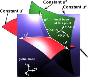
Fig. 1 - Coordinate surfaces, coordinate lines, and coordinate axes of general curvilinear coordinates.

Αρχείο:Spherical coordinate elements.svg

Fig. 2 - Coordinate surfaces, coordinate lines, and coordinate axes of spherical coordinates. Surfaces: r - spheres, θ - cones, φ - half-planes; Lines: r - straight beams, θ - vertical semicircles, φ - horizontal circles; Axes: r - straight beams, θ - tangents to vertical semicircles, φ - tangents to horizontal circles

For now, consider 3d space. A point P in 3d space can be defined using Cartesian coordinates (x, y, z) [equivalently written (x₁, x₂, x₃)], or in another system (q₁, q₂, q₃), as shown in Fig. 1. The latter is a curvilinear coordinate system, and (q₁, q₂, q₃) are the curvilinear coordinates of the point P.

The surfaces q₁ = constant, q₂ = constant, q₃ = constant are called the coordinate surfaces; and the space curves formed by their intersection in pairs are called the coordinate curves. The coordinate axes are determined by the tangents to the coordinate curves at the intersection of three surfaces. They are not in general fixed directions in space, which happens to be the case for simple Cartesian coordinates.

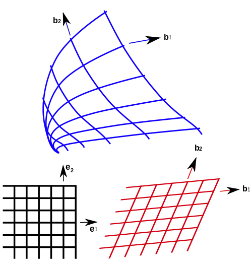
A basis whose vectors change their direction and/or magnitude from point to point is called local basis. All bases associated with curvilinear coordinates are necessarily local. Basis vectors that are the same at all points are global bases, and can be associated only with linear or affine coordinate systems.

Note: usually all basis vectors are denoted by e, for this article e is for the standard basis (Cartesian) and b is for the curvilinear basis.

The relation between the coordinates is given by the invertible transformations:

$x = x(q_1, q_2, q_3),\, y = y(q_1, q_2, q_3),\, z = z(q_1, q_2, q_3)$

$q_1 = q_1(x,y,z),\, q_2 = q_2(x,y,z),\, q_3 = q_3(x,y,z)$

Any point can be written as a position vector r in Cartesian coordinates:

$\mathbf{r} = x \mathbf{e}_x + y\mathbf{e}_y + z\mathbf{e}_z$

where x, y, z are the coordinates of the position vector with respect to the standard basis vectors e_{x, ey, ez.}

However, in a general curvilinear system, there may well not be any natural global basis vectors. Instead, we note that in the Cartesian system, we have the property that

$\mathbf{e}_x = \dfrac{\partial\mathbf{r}}{\partial x}; \; \mathbf{e}_y = \dfrac{\partial\mathbf{r}}{\partial y}; \; \mathbf{e}_z = \dfrac{\partial\mathbf{r}}{\partial z}.$

We can apply the same idea to the curvilinear system to determine a system of basis vectors at P. We define

$\mathbf{h}_1 = \dfrac{\partial\mathbf{r}}{\partial q_1}; \; \mathbf{h}_2 = \dfrac{\partial\mathbf{r}}{\partial q_2}; \; \mathbf{h}_3 = \dfrac{\partial\mathbf{r}}{\partial q_3}.$

These may not have unit length, and may also not be orthogonal. In the case that they are orthogonal at all points where the derivatives are well-defined, we define the Lamé coefficients (after Gabriel Lamé) by

$h_1 = |\mathbf{h}_1|; \; h_2 = |\mathbf{h}_2|; \; h_3 = |\mathbf{h}_3|$

and the curvilinear orthonormal basis vectors by

$\mathbf{b}_1 = \dfrac{\mathbf{h}_1}{h_1}; \; \mathbf{b}_2 = \dfrac{\mathbf{h}_2}{h_2}; \; \mathbf{b}_3 = \dfrac{\mathbf{h}_3}{h_3}.$

It is important to note that these basis vectors may well depend upon the position of P; it is therefore necessary that they are not assumed to be constant over a region. (They technically form a basis for the tangent bundle of $\mathbb R^{3}$ at P, and so are local to P.)

In general, curvilinear coordinates allow the generality of basis vectors not all mutually perpendicular to each other, and not required to be of unit length: they can be of arbitrary magnitude and direction. The use of an orthogonal basis makes vector manipulations simpler than for non-orthogonal. However, some areas of physics and engineering, particularly fluid mechanics and continuum mechanics, require non-orthogonal bases to describe deformations and fluid transport to account for complicated directional dependences of physical quantities. A discussion of the general case appears later on this page.

Vector calculus

Πρότυπο:See also

Differential elements

Since the total differential change in r is

$d\mathbf{r}=\dfrac{\partial\mathbf{r}}{\partial q_1}dq_1 + \dfrac{\partial\mathbf{r}}{\partial q_2}dq_2 + \dfrac{\partial\mathbf{r}}{\partial q_3}dq_3 = h_1 dq_1 \mathbf{b}_1 + h_2 dq_2 \mathbf{b}_2 + h_3 dq_3 \mathbf{b}_3$

so scale factors are

$h_i = \left|\frac{\partial\mathbf{r}}{\partial q_i}\right|$

They can also be written for each component of r:

$h^i{}_k = \cfrac{\partial x^i}{\partial q^k}$.

However, this designation is very rarely used, largely replaced with the components of the metric tensor g_ik (see below).

Covariant and contravariant bases

Πρότυπο:Main

Αρχείο:Vector 1-form.svg

A vector v (red) represented by • a vector basis (yellow, left: e₁, e₂, e₃), tangent vectors to coordinate curves (black) and • a covector basis or cobasis (blue, right: e¹, e², e³), normal vectors to coordinate surfaces (grey) in general (not necessarily orthogonal) curvilinear coordinates (q¹, q², q³). Note the basis and cobasis do not coincide unless the coordinate system is orthogonal.

The basis vectors, gradients, and scale factors are all interrelated within a coordinate system by two methods:

Πρότυπο:Ordered list

So depending on the method by which they are built, for a general curvilinear coordinate system there are two sets of basis vectors for every point: {b₁, b₂, b₃} is the covariant basis, and {b¹, b², b³} is the contravariant basis.

A vector v can be given in terms either basis, i.e.,

$\mathbf{v} = v^1\mathbf{b}_1 + v^2\mathbf{b}_2 + v^3\mathbf{b}_3 = v_1\mathbf{b}^1 + v_2\mathbf{b}^2 + v_3\mathbf{b}^3$

The basis vectors relate to the components byΠρότυπο:Rp

$\mathbf{v}\cdot\mathbf{b}^i = v^k\mathbf{b}_k\cdot\mathbf{b}^i = v^k\delta^i_k = v^i$

$\mathbf{v}\cdot\mathbf{b}_i = v_k\mathbf{b}^k\cdot\mathbf{b}_i = v_k\delta_i^k = v_i$

and

$\mathbf{v}\cdot\mathbf{b}_i = v^k\mathbf{b}_k\cdot\mathbf{b}_i = g_{ki}v^k$

$\mathbf{v}\cdot\mathbf{b}^i = v_k\mathbf{b}^k\cdot\mathbf{b}^i = g^{ki}v_k$

where g is the metric tensor (see below).

A vector is covariant or contravariant if, respectively, its components are covariant (lowered indices, written v_k) or contravariant (raised indices, written v^k). From the above vector sums, it can be seen that contravariant vectors are represented with covariant basis vectors, and covariant vectors are represented with contravariant basis vectors.

A key convention in the representation of vectors and tensors in terms of indexed components and basis vectors is invariance in the sense that vector components which transform in a covariant manner (or contravariant manner) are paired with basis vectors that transform in a contravariant manner (or covariant manner).

Covariant basis

Πρότυπο:Main

Constructing a covariant basis in one dimension

Αρχείο:Local basis transformation.svg

Fig. 3 – Transformation of local covariant basis in the case of general curvilinear coordinates

Consider the one-dimensional curve shown in Fig. 3. At point P, taken as an origin, x is one of the Cartesian coordinates, and q¹ is one of the curvilinear coordinates (Fig. 3). The local (non-unit) basis vector is b₁ (notated h₁ above, with b reserved for unit vectors) and it is built on the q¹ axis which is a tangent to that coordinate line at the point P. The axis q¹ and thus the vector b₁ form an angle α with the Cartesian x axis and the Cartesian basis vector e₁.

It can be seen from triangle PAB that

$\cos \alpha = \cfrac{|\mathbf{e}_1|}{|\mathbf{b}_1|} \quad \Rightarrow \quad |\mathbf{e}_1| = |\mathbf{b}_1|\cos \alpha$

where |e₁|, |b₁| are the magnitudes of the two basis vectors, i.e., the scalar intercepts PB and PA. Note that PA is also the projection of b₁ on the x axis.

However, this method for basis vector transformations using directional cosines is inapplicable to curvilinear coordinates for the following reasons:

1. By increasing the distance from P, the angle between the curved line q¹ and Cartesian axis x increasingly deviates from α.
2. At the distance PB the true angle is that which the tangent at point C forms with the x axis and the latter angle is clearly different from α.

The angles that the q¹ line and that axis form with the x axis become closer in value the closer one moves towards point P and become exactly equal at P.

Let point E be located very close to P, so close that the distance PE is infinitesimally small. Then PE measured on the q¹ axis almost coincides with PE measured on the q¹ line. At the same time, the ratio PD/PE (PD being the projection of PE on the x axis) becomes almost exactly equal to cos α.

Let the infinitesimally small intercepts PD and PE be labelled, respectively, as dx and dq¹. Then

$\cos \alpha = \cfrac{dx}{dq^1} = \frac{|\mathbf{e}_1|}{|\mathbf{b}_1|}$.

Thus, the directional cosines can be substituted in transformations with the more exact ratios between infinitesimally small coordinate intercepts. It follows that the component (projection) of b₁ on the x axis is

$p^1 = \mathbf{b}_1\cdot\cfrac{\mathbf{e}_1}{|\mathbf{e}_1|} = |\mathbf{b}_1|\cfrac{|\mathbf{e}_1|}{|\mathbf{e}_1|}\cos\alpha = |\mathbf{b}_1|\cfrac{dx}{dq^1} \quad \Rightarrow \quad \cfrac{p^1}{|\mathbf{b}_1|} = \cfrac{dx}{dq^1}$.

If qⁱ = qⁱ(x₁, x₂, x₃) and x_i = x_i(q¹, q², q³) are smooth (continuously differentiable) functions the transformation ratios can be written as $\cfrac{\partial q^i}{\partial x_j}$ and $\cfrac{\partial x_i}{\partial q^j}$. That is, those ratios are partial derivatives of coordinates belonging to one system with respect to coordinates belonging to the other system.

Constructing a covariant basis in three dimensions

Doing the same for the coordinates in the other 2 dimensions, b₁ can be expressed as:

$\mathbf{b}_1 = p^1\mathbf{e}_1 + p^2\mathbf{e}_2 + p^3\mathbf{e}_3 = \cfrac{\partial x_1}{\partial q^1} \mathbf{e}_1 + \cfrac{\partial x_2}{\partial q^1} \mathbf{e}_2 + \cfrac{\partial x_3}{\partial q^1} \mathbf{e}_3$

Similar equations hold for b₂ and b₃ so that the standard basis {e₁, e₂, e₃} is transformed to a local (ordered and normalised) basis {b₁, b₂, b₃} by the following system of equations:

$\begin{align} \mathbf{b}_1 & = \cfrac{\partial x_1}{\partial q^1} \mathbf{e}_1 + \cfrac{\partial x_2}{\partial q^1} \mathbf{e}_2 + \cfrac{\partial x_3}{\partial q^1} \mathbf{e}_3 \\ \mathbf{b}_2 & = \cfrac{\partial x_1}{\partial q^2} \mathbf{e}_1 + \cfrac{\partial x_2}{\partial q^2} \mathbf{e}_2 + \cfrac{\partial x_3}{\partial q^2} \mathbf{e}_3 \\ \mathbf{b}_3 & = \cfrac{\partial x_1}{\partial q^3} \mathbf{e}_1 + \cfrac{\partial x_2}{\partial q^3} \mathbf{e}_2 + \cfrac{\partial x_3}{\partial q^3} \mathbf{e}_3 \end{align}$

By analogous reasoning, one can obtain the inverse transformation from local basis to standard basis:

$\begin{align} \mathbf{e}_1 & = \cfrac{\partial q^1}{\partial x_1} \mathbf{b}_1 + \cfrac{\partial q^2}{\partial x_1} \mathbf{b}_2 + \cfrac{\partial q^3}{\partial x_1} \mathbf{b}_3 \\ \mathbf{e}_2 & = \cfrac{\partial q^1}{\partial x_2} \mathbf{b}_1 + \cfrac{\partial q^2}{\partial x_2} \mathbf{b}_2 + \cfrac{\partial q^3}{\partial x_2} \mathbf{b}_3 \\ \mathbf{e}_3 & = \cfrac{\partial q^1}{\partial x_3} \mathbf{b}_1 + \cfrac{\partial q^2}{\partial x_3} \mathbf{b}_2 + \cfrac{\partial q^3}{\partial x_3} \mathbf{b}_3 \end{align}$

Jacobian of the transformation

The above systems of linear equations can be written in matrix form as

$\cfrac{\partial x_i}{\partial q^k} \mathbf{e}_i = \mathbf{b}_k, \quad \cfrac{\partial q^i}{\partial x_k} \mathbf{b}_i = \mathbf{e}_k$.

This coefficient matrix of the linear system is the Jacobian matrix (and its inverse) of the transformation. These are the equations that can be used to transform a Cartesian basis into a curvilinear basis, and vice versa.

In three dimensions, the expanded forms of these matrices are

$\mathbf{J} = \begin{bmatrix} \cfrac{\partial x_1}{\partial q^1} & \cfrac{\partial x_1}{\partial q^2} & \cfrac{\partial x_1}{\partial q^3} \\ \cfrac{\partial x_2}{\partial q^1} & \cfrac{\partial x_2}{\partial q^2} & \cfrac{\partial x_2}{\partial q^3} \\ \cfrac{\partial x_3}{\partial q^1} & \cfrac{\partial x_3}{\partial q^2} & \cfrac{\partial x_3}{\partial q^3} \\ \end{bmatrix},\quad \mathbf{J}^{-1} = \begin{bmatrix} \cfrac{\partial q^1}{\partial x_1} & \cfrac{\partial q^1}{\partial x_2} & \cfrac{\partial q^1}{\partial x_3} \\ \cfrac{\partial q^2}{\partial x_1} & \cfrac{\partial q^2}{\partial x_2} & \cfrac{\partial q^2}{\partial x_3} \\ \cfrac{\partial q^3}{\partial x_1} & \cfrac{\partial q^3}{\partial x_2} & \cfrac{\partial q^3}{\partial x_3} \\ \end{bmatrix}$

In the inverse transformation (second equation system), the unknowns are the curvilinear basis vectors. For all points there can only exist one and only one set of basis vectors (else vectors are not well defined at those points). This condition is satisfied if and only if the equation system has a single solution, from linear algebra, a linear equation system has a single solution (non-trivial) only if the determinant of its system matrix is non-zero:

$\det(\mathbf{J}^{-1}) \neq 0$

which shows the rationale behind the above requirement concerning the inverse Jacobian determinant.

Generalization to n dimensions

The formalism extends to any finite dimension as follows.

Consider the real Euclidean n-dimensional space, that is Rⁿ = R × R × ... × R (n times) where R is the set of real numbers and × denotes the Cartesian product, which is a vector space.

The coordinates of this space can be denoted by: x = (x₁, x₂,...,x_n). Since this is a vector (an element of the vector space), it can be written as:

$\mathbf{x} = \sum_{i=1}^n x_i\mathbf{e}^i$

where e¹ = (1,0,0...,0), e² = (0,1,0...,0), e³ = (0,0,1...,0),...,eⁿ = (0,0,0...,1) is the standard basis set of vectors for the space Rⁿ, and i = 1, 2,...n is an index labelling components. Each vector has exactly one component in each dimension (or "axis") and they are mutually orthogonal (perpendicular) and normalized (has unit magnitude).

More generally, we can define basis vectors b_i so that they depend on q = (q₁, q₂,...,q_n), i.e. they change from point to point: b_i = b_i(q). In which case to define the same point x in terms of this alternative basis: the coordinates with respect to this basis v_i also necessarily depend on x also, that is v_i = v_i(x). Then a vector v in this space, with respect to these alternative coordinates and basis vectors, can be expanded as a linear combination in this basis (which simply means to multiply each basis vector e_i by a number v_i – scalar multiplication):

$\mathbf{v} = \sum_{j=1}^n \bar{v}^j\mathbf{b}_j = \sum_{j=1}^n \bar{v}^j(\mathbf{q})\mathbf{b}_j(\mathbf{q})$

The vector sum that describes v in the new basis is composed of different vectors, although the sum itself remains the same.

Transformation of coordinates

From a more general and abstract perspective, a curvilinear coordinate system is simply a coordinate patch on the differentiable manifold Eⁿ (n-dimensional Euclidian space) that is diffeomorphic to the Cartesian coordinate patch on the manifold. Note that two diffeomorphic coordinate patches on a differential manifold need not overlap differentiably. With this simple definition of a curvilinear coordinate system, all the results that follow below are simply applications of standard theorems in differential topology.

The transformation functions are such that there's a one-to-one relationship between points in the "old" and "new" coordinates, that is, those functions are bijections, and fulfil the following requirements within their domains: Πρότυπο:Ordered list

Vector and tensor algebra in three-dimensional curvilinear coordinates

Πρότυπο:Einstein summation convention Elementary vector and tensor algebra in curvilinear coordinates is used in some of the older scientific literature in mechanics and physics and can be indispensable to understanding work from the early and mid-1900s, for example the text by Green and Zerna. Some useful relations in the algebra of vectors and second-order tensors in curvilinear coordinates are given in this section. The notation and contents are primarily from Ogden, Naghdi, Simmonds, Green and Zerna, Basar and Weichert, and Ciarlet.

Tensors in curvilinear coordinates

A second-order tensor can be expressed as

$\boldsymbol{S} = S^{ij}\mathbf{b}_i\otimes\mathbf{b}_j = S^i{}_j\mathbf{b}_i\otimes\mathbf{b}^j = S_i{}^j\mathbf{b}^i\otimes\mathbf{b}_j = S_{ij}\mathbf{b}^i\otimes\mathbf{b}^j$

where $\scriptstyle\otimes$ denotes the tensor product. The components S^ij are called the contravariant components, Sⁱ _j the mixed right-covariant components, S_i ^j the mixed left-covariant components, and S_ij the covariant components of the second-order tensor. The components of the second-order tensor are related by

$S^{ij} = g^{ik}S_k{}^j = g^{jk}S^i{}_k = g^{ik}g^{j\ell}S_{k\ell}$

The metric tensor in orthogonal curvilinear coordinates

Πρότυπο:Main

At each point, one can construct a small line element dx, so the square of the length of the line element is the scalar product dx • dx and is called the metric of the space, given by:

$d\mathbf{x}\cdot d\mathbf{x} = \cfrac{\partial x_i}{\partial q^j}\cfrac{\partial x_i}{\partial q^k}dq^jdq^k$

and the symmetric quantity

$g_{ij}(q^i,q^j) = \cfrac{\partial x_k}{\partial q^i}\cfrac{\partial x_k}{\partial q^j} = \mathbf{b}_i\cdot\mathbf{b}_j$

is called the fundamental (or metric) tensor of the Euclidean space in curvilinear coordinates.

Indices can be raised and lowered by the metric:

$v^i = g^{ik}v_k$

Relation to Lamé coefficients

Defining the scale factors h_ij by

$h_ih_j = g_{ij} = \mathbf{b}_i\cdot\mathbf{b}_j \quad \Rightarrow \quad h_i =\sqrt{g_{ii}}= \left|\mathbf{b}_i\right|=\left|\cfrac{\partial\mathbf{x}}{\partial q^i}\right|$

gives a relation between the metric tensor and the Lamé coefficients. Note also that

$g_{ij} = \cfrac{\partial\mathbf{x}}{\partial q^i}\cdot\cfrac{\partial\mathbf{x}}{\partial q^j} = \left( h_{ki}\mathbf{e}_k\right)\cdot\left( h_{mj}\mathbf{e}_m\right) = h_{ki}h_{kj}$

where h_ij are the Lamé coefficients. For an orthogonal basis we also have:

$g = g_{11}g_{22}g_{33} = h_1^2h_2^2h_3^2 \quad \Rightarrow \quad \sqrt{g} = h_1h_2h_3 = J$

Example: Polar coordinates

If we consider polar coordinates for R², note that

$(x, y)=(r \cos \theta, r \sin \theta) \,\!$

(r, θ) are the curvilinear coordinates, and the Jacobian determinant of the transformation (r,θ) → (r cos θ, r sin θ) is r.

The orthogonal basis vectors are b_r = (cos θ, sin θ), b_θ = (−r sin θ, r cos θ). The normalized basis vectors are e_r = (cos θ, sin θ), e_θ = (−sin θ, cos θ) and the scale factors are h_r = 1 and h_θ= r. The fundamental tensor is g₁₁ =1, g₂₂ =r², g₁₂ = g₂₁ =0.

The alternating tensor

In an orthonormal right-handed basis, the third-order alternating tensor is defined as

$\boldsymbol{\mathcal{E}} = \epsilon_{ijk}\mathbf{e}^i\otimes\mathbf{e}^j\otimes\mathbf{e}^k$

In a general curvilinear basis the same tensor may be expressed as

$\boldsymbol{\mathcal{E}} = \mathcal{E}_{ijk}\mathbf{b}^i\otimes\mathbf{b}^j\otimes\mathbf{b}^k = \mathcal{E}^{ijk}\mathbf{b}_i\otimes\mathbf{b}_j\otimes\mathbf{b}_k$

It can also be shown that

$\mathcal{E}^{ijk} = \cfrac{1}{J}\epsilon_{ijk} = \cfrac{1}{+\sqrt{g}}\epsilon_{ijk}$

Christoffel symbols

Christoffel symbols of the first kind

$\mathbf{b}_{i,j} = \frac{\partial \mathbf{b}_i}{\partial q^j} = \Gamma_{ijk}\mathbf{b}^k \quad \Rightarrow \quad \mathbf{b}_{i,j} \cdot \mathbf{b}_k = \Gamma_{ijk}$

where the comma denotes a partial derivative (see Ricci calculus). To express Γ_ijk in terms of g_ij we note that

$\begin{align} g_{ij,k} & = (\mathbf{b}_i\cdot\mathbf{b}_j)_{,k} = \mathbf{b}_{i,k}\cdot\mathbf{b}_j + \mathbf{b}_i\cdot\mathbf{b}_{j,k} = \Gamma_{ikj} + \Gamma_{jki}\\ g_{ik,j} & = (\mathbf{b}_i\cdot\mathbf{b}_k)_{,j} = \mathbf{b}_{i,j}\cdot\mathbf{b}_k + \mathbf{b}_i\cdot\mathbf{b}_{k,j} = \Gamma_{ijk} + \Gamma_{kji}\\ g_{jk,i} & = (\mathbf{b}_j\cdot\mathbf{b}_k)_{,i} = \mathbf{b}_{j,i}\cdot\mathbf{b}_k + \mathbf{b}_j\cdot\mathbf{b}_{k,i} = \Gamma_{jik} + \Gamma_{kij} \end{align}$

Since

$\mathbf{b}_{i,j} = \mathbf{b}_{j,i}\quad\Rightarrow\quad\Gamma_{ijk} = \Gamma_{jik}$

using these to rearrange the above relations gives

$\Gamma_{ijk} = \frac{1}{2}(g_{ik,j} + g_{jk,i} - g_{ij,k}) = \frac{1}{2}[(\mathbf{b}_i\cdot\mathbf{b}_k)_{,j} + (\mathbf{b}_j\cdot\mathbf{b}_k)_{,i} - (\mathbf{b}_i\cdot\mathbf{b}_j)_{,k}]$

Christoffel symbols of the second kind

$\Gamma_{ij}{}^k = \Gamma_{ji}{}^k,\quad \cfrac{\partial \mathbf{b}_i}{\partial q^j} = \Gamma_{ij}{}^k\mathbf{b}_k$

This implies that

$\Gamma_{ij}{}^k = \cfrac{\partial \mathbf{b}_i}{\partial q^j}\cdot\mathbf{b}^k = -\mathbf{b}_i\cdot\cfrac{\partial \mathbf{b}^k}{\partial q^j}$

Other relations that follow are

$\cfrac{\partial \mathbf{b}^i}{\partial q^j} = -\Gamma^i{}_{jk}\mathbf{b}^k,\quad \boldsymbol{\nabla}\mathbf{b}_i = \Gamma_{ij}{}^k\mathbf{b}_k\otimes\mathbf{b}^j,\quad \boldsymbol{\nabla}\mathbf{b}^i = -\Gamma_{jk}{}^i\mathbf{b}^k\otimes\mathbf{b}^j$

Vector operations

Πρότυπο:Ordered list

Vector and tensor calculus in three-dimensional curvilinear coordinates

Πρότυπο:Einstein summation convention

Adjustments need to be made in the calculation of line, surface and volume integrals. For simplicity, the following restricts to three dimensions and orthogonal curvilinear coordinates. However, the same arguments apply for n-dimensional spaces. When the coordinate system is not orthogonal, there are some additional terms in the expressions.

Simmonds, in his book on tensor analysis, quotes Albert Einstein saying

The magic of this theory will hardly fail to impose itself on anybody who has truly understood it; it represents a genuine triumph of the method of absolute differential calculus, founded by Gauss, Riemann, Ricci, and Levi-Civita.

Vector and tensor calculus in general curvilinear coordinates is used in tensor analysis on four-dimensional curvilinear manifolds in general relativity, in the mechanics of curved shells, in examining the invariance properties of Maxwell's equations which has been of interest in metamaterials and in many other fields.

Some useful relations in the calculus of vectors and second-order tensors in curvilinear coordinates are given in this section. The notation and contents are primarily from Ogden, Simmonds, Green and Zerna, Basar and Weichert, and Ciarlet.

Let φ = φ(x) be a well defined scalar field and v = v(x) a well-defined vector field, and λ₁, λ₂... be parameters of the coordinates

Geometric elements

Πρότυπο:Ordered list

Integration

Operator	Scalar field	Vector field
Line integral	$\int_C \varphi(\mathbf{x}) ds = \int_a^b \varphi(\mathbf{x}(\lambda))\left|{\partial \mathbf{x} \over \partial \lambda}\right| d\lambda$	$\int_C \mathbf{v}(\mathbf{x}) \cdot d\mathbf{s} = \int_a^b \mathbf{v}(\mathbf{x}(\lambda))\cdot\left({\partial \mathbf{x} \over \partial \lambda}\right) d\lambda$
Surface integral	$\int_S \varphi(\mathbf{x}) dS = \iint_T \varphi(\mathbf{x}(\lambda_1, \lambda_2)) \left|{\partial \mathbf{x} \over \partial \lambda_1}\times {\partial \mathbf{x} \over \partial \lambda_2}\right| d\lambda_1 d\lambda_2$	$\int_S \mathbf{v}(\mathbf{x}) \cdot dS = \iint_T \mathbf{v}(\mathbf{x}(\lambda_1, \lambda_2)) \cdot\left({\partial \mathbf{x} \over \partial \lambda_1}\times {\partial \mathbf{x} \over \partial \lambda_2}\right) d\lambda_1 d\lambda_2$
Volume integral	$\iiint_V \varphi(x,y,z) dV = \iiint_V \chi(q_1,q_2,q_3) Jdq_1dq_2dq_3$	$\iiint_V \mathbf{u}(x,y,z) dV = \iiint_V \mathbf{v}(q_1,q_2,q_3) Jdq_1dq_2dq_3$

Differentiation

The expressions for the gradient, divergence, and Laplacian can be directly extended to n-dimensions, however the curl is only defined in 3d.

The vector field b_i is tangent to the qⁱ coordinate curve and forms a natural basis at each point on the curve. This basis, as discussed at the beginning of this article, is also called the covariant curvilinear basis. We can also define a reciprocal basis, or contravariant curvilinear basis, bⁱ. All the algebraic relations between the basis vectors, as discussed in the section on tensor algebra, apply for the natural basis and its reciprocal at each point x.

Operator	Scalar field	Vector field	2nd order tensor field
Gradient	$\nabla\varphi = \cfrac{1}{h_i}{\partial\varphi \over \partial q^i} \mathbf{b}^i$	$\nabla\mathbf{v} = \cfrac{1}{h_i^2}{\partial \mathbf{v} \over \partial q^i}\otimes\mathbf{b}_i$	$\boldsymbol{\nabla}\boldsymbol{S} = \cfrac{\partial \boldsymbol{S}}{\partial q^i}\otimes\mathbf{b}^i$
Divergence	N/A	$\nabla \cdot \mathbf{v} = \cfrac{1}{\prod_j h_j} \frac{\partial }{\partial q^i}(v^i\prod_{j\ne i} h_j)$	$(\boldsymbol{\nabla}\cdot\boldsymbol{S})\cdot\mathbf{a} = \boldsymbol{\nabla}\cdot(\boldsymbol{S}\cdot\mathbf{a})$ where a is an arbitrary constant vector. In curvilinear coordinates, $\boldsymbol{\nabla}\cdot\boldsymbol{S} = \left[\cfrac{\partial S_{ij}}{\partial q^k} - \Gamma^l_{ki}S_{lj} - \Gamma^l_{kj}S_{il}\right]g^{ik}\mathbf{b}^j$
Laplacian	$\nabla^2 \varphi = \cfrac{1}{h_1h_2h_3}\frac{\partial }{\partial q^i}\left(\cfrac{h_1h_2h_3}{h_i^2}\frac{\partial \varphi}{\partial q^i}\right)$
Curl	N/A	For vector fields in 3d only, $\nabla\times\mathbf{v} = \frac{1}{h_1h_2h_3} \mathbf{e}_i \epsilon_{ijk} h_i \frac{\partial (h_k v_k)}{\partial q^j}$ where $\epsilon_{ijk}$ is the Levi-Civita symbol.	N/A

Fictitious forces in general curvilinear coordinates

An inertial coordinate system is defined as a system of space and time coordinates x₁, x₂, x₃, t in terms of which the equations of motion of a particle free of external forces are simply d²x_j/dt² = 0. In this context, a coordinate system can fail to be “inertial” either due to non-straight time axis or non-straight space axes (or both). In other words, the basis vectors of the coordinates may vary in time at fixed positions, or they may vary with position at fixed times, or both. When equations of motion are expressed in terms of any non-inertial coordinate system (in this sense), extra terms appear, called Christoffel symbols. Strictly speaking, these terms represent components of the absolute acceleration (in classical mechanics), but we may also choose to continue to regard d²x_j/dt² as the acceleration (as if the coordinates were inertial) and treat the extra terms as if they were forces, in which case they are called fictitious forces. The component of any such fictitious force normal to the path of the particle and in the plane of the path’s curvature is then called centrifugal force.

This more general context makes clear the correspondence between the concepts of centrifugal force in rotating coordinate systems and in stationary curvilinear coordinate systems. (Both of these concepts appear frequently in the literature.) For a simple example, consider a particle of mass m moving in a circle of radius r with angular speed w relative to a system of polar coordinates rotating with angular speed W. The radial equation of motion is mr” = F_r + mr(w + W)². Thus the centrifugal force is mr times the square of the absolute rotational speed A = w + W of the particle. If we choose a coordinate system rotating at the speed of the particle, then W = A and w = 0, in which case the centrifugal force is mrA², whereas if we choose a stationary coordinate system we have W = 0 and w = A, in which case the centrifugal force is again mrA². The reason for this equality of results is that in both cases the basis vectors at the particle’s location are changing in time in exactly the same way. Hence these are really just two different ways of describing exactly the same thing, one description being in terms of rotating coordinates and the other being in terms of stationary curvilinear coordinates, both of which are non-inertial according to the more abstract meaning of that term.

When describing general motion, the actual forces acting on a particle are often referred to the instantaneous osculating circle tangent to the path of motion, and this circle in the general case is not centered at a fixed location, and so the decomposition into centrifugal and Coriolis components is constantly changing. This is true regardless of whether the motion is described in terms of stationary or rotating coordinates.

Εσωτερική Αρθρογραφία

• Σύστημα Συντεταγμένων
• Σύστημα Αναφοράς
• Πολικές Συντεταγμένες
• Κυλινδρικές Συντεταγμένες
• Σφαιρικές Συντεταγμένες
• Καμπυλόγραμμες Συντεταγμένες
• Covariance and contravariance
• Basic introduction to the mathematics of curved spacetime
• Orthogonal coordinates
• Frenet–Serret formulas
• Covariant derivative
• Tensor derivative (continuum mechanics)
• Curvilinear perspective
• Del in cylindrical and spherical coordinates

Βιβλιογραφία

• Spiegel, M. R. (1959). Vector Analysis. New York: Schaum's Outline Series. ISBN 0-07-084378-3. 
• Arfken, George (1995). Mathematical Methods for Physicists. Academic Press. ISBN 0-12-059877-9. 

Ιστογραφία

• Ομώνυμο άρθρο στην Βικιπαίδεια
• Ομώνυμο άρθρο στην Livepedia
• Derivation of Unit Vectors in Curvilinear Coordinates
• MathWorld's page on Curvilinear Coordinates
• Prof. R. Brannon's E-Book on Curvilinear Coordinates
• [1] – Wikiversity, Introduction to Elasticity/Tensors.
• [ ]
• [ ]

Κίνδυνοι Χρήσης

Αν και θα βρείτε εξακριβωμένες πληροφορίες σε αυτήν την εγκυκλοπαίδεια ωστόσο, παρακαλούμε να λάβετε σοβαρά υπ' όψη ότι η "Sciencepedia" δεν μπορεί να εγγυηθεί, από καμιά άποψη, την εγκυρότητα των πληροφοριών που περιλαμβάνει. "Οι πληροφορίες αυτές μπορεί πρόσφατα να έχουν αλλοιωθεί, βανδαλισθεί ή μεταβληθεί από κάποιο άτομο, η άποψη του οποίου δεν συνάδει με το "επίπεδο γνώσης" του ιδιαίτερου γνωστικού τομέα που σας ενδιαφέρει." Πρέπει να λάβετε υπ' όψη ότι όλα τα άρθρα μπορεί να είναι ακριβή, γενικώς, και για μακρά χρονική περίοδο, αλλά να υποστούν κάποιο βανδαλισμό ή ακατάλληλη επεξεργασία, ελάχιστο χρονικό διάστημα, πριν τα δείτε. Επίσης, Οι διάφοροι "Εξωτερικοί Σύνδεσμοι (Links)" (όχι μόνον, της Sciencepedia αλλά και κάθε διαδικτυακού ιστότοπου (ή αλλιώς site)), αν και άκρως απαραίτητοι, είναι αδύνατον να ελεγχθούν (λόγω της ρευστής φύσης του Web), και επομένως είναι ενδεχόμενο να οδηγήσουν σε παραπλανητικό, κακόβουλο ή άσεμνο περιεχόμενο. Ο αναγνώστης πρέπει να είναι εξαιρετικά προσεκτικός όταν τους χρησιμοποιεί.

- Μην κάνετε χρήση του περιεχομένου της παρούσας εγκυκλοπαίδειας
αν διαφωνείτε με όσα αναγράφονται σε αυτήν

---

>>Διαμαρτυρία προς την wikia<<

- Όχι, στις διαφημίσεις που περιέχουν απαράδεκτο περιεχόμενο (άσεμνες εικόνες, ροζ αγγελίες κλπ.)

---