Διαφορική Μορφή

Διαφορική Μορφή

Differential Form

Διαφορική Μορφή
Διανυσματικό Πεδίο
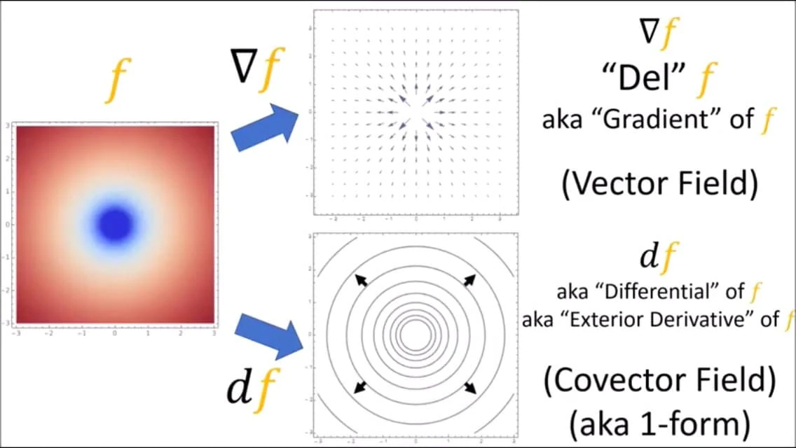
Κλίση

Διαφορική Μορφή

Διαφορική Μορφή

Delta του Cartan

Διαφορική Τοπολογία
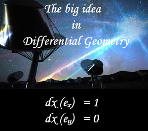
Διαφορική Γεωμετρία

---

Διαφορική Μορφή
Μοναδιαίο Διάνυσμα

- Ένα Μαθηματικό Δόμημα

Ετυμολογία

Η ονομασία "Διαφορική" σχετίζεται ετυμολογικά με την λέξη "Διαφόριση".

Ορισμός

$\omega: U\rightarrow\bigoplus_{p \in U} T^*_p(\mathbb{R}^n)$ $p \in U \mapsto \omega_p \in T^*_p(\mathbb{R}^n)$

Εισαγωγή

In the mathematical fields of differential geometry and tensor calculus, differential forms are an approach to multivariable calculus that is independent of coordinates. Differential forms provide a unified approach to defining integrands over curves, surfaces, volumes, and higher dimensional manifolds. The modern notion of differential forms was pioneered by Élie Cartan. It has many applications, especially in geometry, topology and physics.

For instance, the expression f(x) dx from one-variable calculus is called a 1-form, and can be integrated over an interval [a,b] in the domain of f:

$\int_a^b f(x) \,dx$

and similarly the expression: f(x,y,z) dx∧dy + g(x,y,z) dx∧dz + h(x,y,z) dy∧dz is a 2-form that has a surface integral over an oriented surface S:

$\int_S f(x,y,z)\,dx\wedge dy + g(x,y,z)\,dx\wedge dz + h(x,y,z)\,dy\wedge dz.$

Likewise, a 3-form f(x, y, z) dx∧dy∧dz represents a volume element that can be integrated over a region of space.

The algebra of differential forms is organized in a way that naturally reflects the orientation of the domain of integration. There is an operation d on differential forms known as the exterior derivative that, when acting on a k-form produces a (k+1)-form. This operation extends the differential of a function, and the divergence and the curl of a vector field in an appropriate sense that makes the fundamental theorem of calculus, the divergence theorem, Green's theorem, and Stokes' theorem special cases of the same general result, known in this context also as the general Stokes' theorem. In a deeper way, this theorem relates the topology of the domain of integration to the structure of the differential forms themselves; the precise connection is known as De Rham's theorem.

The general setting for the study of differential forms is on a differentiable manifold. Differential 1-forms are naturally dual to vector fields on a manifold, and the pairing between vector fields and 1-forms is extended to arbitrary differential forms by the interior product. The algebra of differential forms along with the exterior derivative defined on it is preserved by the pullback under smooth functions between two manifolds. This feature allows geometrically invariant information to be moved from one space to another via the pullback, provided the information is expressed in terms of differential forms. As an example, the change of variables formula for integration becomes a simple statement that an integral is preserved under pullback.

History

Differential forms are part of the field of differential geometry, influenced by linear algebra. Although the notion of a differential is quite old, the initial attempt at an algebraic organization of differential forms is usually credited to Élie Cartan in his 1899 paper.

Concept

Differential forms provide an approach to multivariable calculus that is independent of coordinates.

Let U be an open set in Rⁿ. A differential 0-form ("zero form") is defined to be a smooth function f on U. If v is any vector in Rⁿ, then f has a directional derivative ∂_v f, which is another function on U whose value at a point p ∈ U is the rate of change (at p) of f in the v direction:

$(\partial_v f)(p) = \frac{d}{dt} f(p+tv)\Big|_{t=0}.$

(This notion can be extended to the case that v is a vector field on U by evaluating v at the point p in the definition.)

In particular, if v = e_j is the jth coordinate vector then ∂_vf is the partial derivative of f with respect to the jth coordinate function, i.e., ∂f / ∂x^j, where x¹, x², ... xⁿ are the coordinate functions on U. By their very definition, partial derivatives depend upon the choice of coordinates: if new coordinates y¹, y², ... yⁿ are introduced, then

$\frac{\partial f}{\partial x^j} = \sum_{i=1}^n\frac{\partial y^i}{\partial x^j}\frac{\partial f}{\partial y^i}$

The first idea leading to differential forms is the observation that ∂_v f (p) is a linear function of v:

$(\partial_{v+w} f)(p) = (\partial_v f)(p) + (\partial_w f)(p)$

$(\partial_{c v} f)(p) = c (\partial_v f)(p)$

for any vectors v, w and any real number c. This linear map from Rⁿ to R is denoted df_p and called the derivative of f at p. Thus df_p(v) = ∂_v f (p). The object df can be viewed as a function on U, whose value at p is not a real number, but the linear map df_p. This is just the usual Fréchet derivative — an example of a differential 1-form.

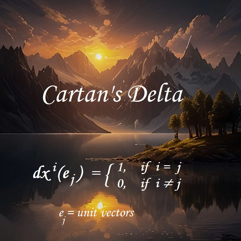
Since any vector v is a linear combination ∑ v^je_j of its components, df is uniquely determined by df_p(e_j) for each j and each p∈U, which are just the partial derivatives of f on U. Thus df provides a way of encoding the partial derivatives of f. It can be decoded by noticing that the coordinates x¹, x²,... xⁿ are themselves functions on U, and so define differential 1-forms dx¹, dx², ..., dxⁿ. Since ∂xⁱ / ∂x^j = δ_ij, the Kronecker delta function, it follows that

Πρότυπο:NumBlk

The meaning of this expression is given by evaluating both sides at an arbitrary point p: on the right hand side, the sum is defined "pointwise", so that

$df_p = \sum_{i=1}^n \frac{\partial f}{\partial x^i}(p) (dx^i)_p .$

Applying both sides to e_j, the result on each side is the jth partial derivative of f at p. Since p and j were arbitrary, this proves the formula Πρότυπο:EquationNote.

More generally, for any smooth functions g_i and h_i on U, we define the differential 1-form α = ∑_i g_i dh_i pointwise by

$\alpha_p = \sum_i g_i(p) (dh_i)_p\,\!$

for each p ∈ U. Any differential 1-form arises this way, and by using Πρότυπο:EquationNote it follows that any differential 1-form α on U may be expressed in coordinates as

$\alpha = \sum_{i=1}^n f_i\, dx^i$

for some smooth functions f_i on U.

The second idea leading to differential forms arises from the following question: given a differential 1-form α on U, when does there exist a function f on U such that α = df? The above expansion reduces this question to the search for a function f whose partial derivatives ∂f / ∂xⁱ are equal to n given functions f_i. For n>1, such a function does not always exist: any smooth function f satisfies

$\frac{\partial^2 f}{\partial x^i \, \partial x^j} = \frac{\partial^2 f}{\partial x^j \, \partial x^i}$

so it will be impossible to find such an f unless

$\frac{\partial f_j}{\partial x^i} - \frac{\partial f_i}{\partial x^j}=0.$

for all i and j.

The skew-symmetry of the left hand side in i and j suggests introducing an antisymmetric product $\wedge$ on differential 1-forms, the wedge product, so that these equations can be combined into a single condition

$\sum_{i,j=1}^n \frac{\partial f_j}{\partial x^i} dx^i \wedge dx^j = 0$

where

$dx^i \wedge dx^j = - dx^j \wedge dx^i. \,$

This is an example of a differential 2-form: the exterior derivative dα of α= ∑_j=1ⁿ f_j dx^j is given by

$d\alpha = \sum_{j=1}^n df_j \wedge dx^j = \sum_{i,j=1}^n \frac{\partial f_j}{\partial x^i} dx^i \wedge dx^j.$

To summarize: dα = 0 is a necessary condition for the existence of a function f with α = df.

Differential 0-forms, 1-forms, and 2-forms are special cases of differential forms. For each k, there is a space of differential k-forms, which can be expressed in terms of the coordinates as

$\sum_{i_1,i_2\ldots i_k=1}^n f_{i_1i_2\ldots i_k} dx^{i_1} \wedge dx^{i_2} \wedge\cdots \wedge dx^{i_k}$

for a collection of functions f_{i1i2 ... ik}. (Of course, as assumed below, one can restrict the sum to the case $i_1<i_2<\cdots <i_{k-1}<i_k\,$.)

Differential forms can be multiplied together using the wedge product, and for any differential k-form α, there is a differential (k + 1)-form dα called the exterior derivative of α.

Differential forms, the wedge product and the exterior derivative are independent of a choice of coordinates. Consequently they may be defined on any smooth manifold M. One way to do this is cover M with coordinate charts and define a differential k-form on M to be a family of differential k-forms on each chart which agree on the overlaps. However, there are more intrinsic definitions which make the independence of coordinates manifest.

Intrinsic definitions

Let M be a smooth manifold. A differential form of degree k is a smooth section of the kth exterior power of the cotangent bundle of M. At any point p∈M, a k-form β defines an alternating multilinear map

$\beta_p\colon T_p M\times \cdots \times T_p M \to \mathbb{R}$

(with k factors of T_pM in the product), where T_pM is the tangent space to M at p. Equivalently, β is a totally antisymmetric covariant tensor field of rank k.

The set of all differential k-forms on a manifold M is a vector space, often denoted Ω^k(M).

For example, a differential 1-form α assigns to each point p∈M a linear functional α_p on T_pM. In the presence of an inner product on T_pM (induced by a Riemannian metric on M), α_p may be represented as the inner product with a tangent vector X_p. Differential 1-forms are sometimes called covariant vector fields, covector fields, or "dual vector fields", particularly within physics.

Operations

There are several operations on differential forms: the wedge product of two differential forms, the exterior derivative of a single differential form, the interior product of a differential form and a vector field, and the Lie derivative of a differential form with respect to a vector field.

Wedge product

The wedge product of a k-form α and an l-form β is a (k + l)-form denoted αΛβ. For example, if k = l = 1, then αΛβ is the 2-form whose value at a point p is the alternating bilinear form defined by

$(\alpha\wedge\beta)_p(v,w)=\alpha_p(v)\beta_p(w) - \alpha_p(w)\beta_p(v)$

for v, w ∈ T_pM. (In an alternative convention, the right hand side is divided by two in this formula.)

The wedge product is bilinear: for instance, if α, β, and γ are any differential forms, then

$\alpha \wedge (\beta + \gamma) = \alpha \wedge \beta + \alpha \wedge \gamma.$

It is skew commutative (also known as graded commutative), meaning that it satisfies a variant of anticommutativity that depends on the degrees of the forms: if α is a k-form and β is an l-form, then

$\alpha \wedge \beta = (-1)^{kl} \beta \wedge \alpha. \,$

Riemannian manifold

On a Riemannian manifold, or more generally a pseudo-Riemannian manifold, vector fields and covector field can be identified (the metric is a fiber-wise isomorphism of the tangent space and the cotangent space), and additional operations can thus be defined, such as the Hodge star operator $*\colon \Omega^k(M) \overset{\sim}{\to} \Omega^{n-k}(M)$ and codifferential $\delta\colon \Omega^k(M)\rightarrow \Omega^{k-1}(M),$ (degree $-1$) which is adjoint to the exterior differential d.

Vector field structures

On a pseudo-Riemannian manifold, 1-forms can be identified with vector fields; vector fields have additional distinct algebraic structures, which are listed here for context and to avoid confusion.

Firstly, each (co)tangent space generates a Clifford algebra, where the product of a (co)vector with itself is given by the value of a quadratic form - in this case, the natural one induced by the metric. This algebra is distinct from the exterior algebra of differential forms, which can be viewed as a Clifford algebra where the quadratic form vanishes (since the exterior product of any vector with itself is zero). Clifford algebras are thus non-anti-commutative ("quantum") deformations of the exterior algebra. They are studied in geometric algebra.

Another alternative is to consider vector fields as derivations, and consider the (noncommutative) algebra of differential operators they generate, which is the Weyl algebra, and is a noncommutative ("quantum") deformation of the symmetric algebra in the vector fields.

Exterior differential complex

One important property of the exterior derivative is that d² = 0. This means that the exterior derivative defines a cochain complex:

$0 \to\Omega^0(M)\ \stackrel{d}{\to}\ \Omega^1(M)\ \stackrel{d}{\to}\ \Omega^2(M)\ \stackrel{d}{\to}\ \Omega^3(M) \to \cdots \ \to\ \Omega^n(M)\ \to \ 0.$

By the Poincaré lemma, this complex is locally exact except at Ω⁰(M). Its cohomology is the de Rham cohomology of M.

Pullback

Πρότυπο:See also

One of the main reasons the cotangent bundle rather than the tangent bundle is used in the construction of the exterior complex is that differential forms are capable of being pulled back by smooth maps, while vector fields cannot be pushed forward by smooth maps unless the map is, say, a diffeomorphism. The existence of pullback homomorphisms in de Rham cohomology depends on the pullback of differential forms.

Differential forms can be moved from one manifold to another using a smooth map. If f : M → N is smooth and ω is a smooth k-form on N, then there is a differential form f^*ω on M, called the pullback of ω, which captures the behavior of ω as seen relative to f.

To define the pullback, recall that the differential of f is a map f_* : TM → TN. Fix a differential k-form ω on N. For a point p of M and tangent vectors v₁, ..., v_k to M at p, the pullback of ω is defined by the formula $(f^*\omega)_p(v_1, \ldots, v_k) = \omega_{f(p)}(f_*v_1, \ldots, f_*v_k).$ More abstractly, if ω is viewed as a section of the cotangent bundle T^*N of N, then f^*ω is the section of T^*M defined as the composite map $M \stackrel{f}{\to} N \stackrel{\omega}{\to} T^*N \stackrel{(Df)^*}{\longrightarrow} T^*M.$

Pullback respects all of the basic operations on forms: $f^*(\omega + \eta) = f^*\omega + f^*\eta,$ $f^*(\omega\wedge\eta) = f^*\omega\wedge f^*\eta,$ $f^*(d\omega) = d(f^*\omega).$

The pullback of a form can also be written in coordinates. Assume that x₁, ..., x_m are coordinates on M, that y₁, ..., y_n are coordinates on N, and that these coordinate systems are related by the formulas y_i = f_i(x₁, ..., x_m) for all i. Then, locally on N, ω can be written as

$\omega = \sum_{i_1 < \cdots < i_k} \omega_{i_1\cdots i_k}dy_{i_1} \wedge \cdots \wedge dy_{i_k},$ where, for each choice of i₁, ..., i_k, $\omega_{i_1\cdots i_k}$ is a real-valued function of y₁, ..., y_n. Using the linearity of pullback and its compatibility with wedge product, the pullback of ω has the formula

$f^*\omega = \sum_{i_1 < \cdots < i_k} (\omega_{i_1\cdots i_k}\circ f)df_{i_1}\wedge\cdots\wedge df_{i_n}.$

Each exterior derivative df_i can be expanded in terms of dx₁, ..., dx_m. The resulting k-form can be written using Jacobian matrices:

$f^*\omega = \sum_{i_1 < \cdots < i_k} \sum_{j_1 < \cdots < j_k} (\omega_{i_1\cdots i_k}\circ f)\frac{\partial(f_{i_1}, \ldots, f_{i_k})}{\partial(x_{j_1}, \ldots, x_{j_k})}dx_{j_1} \wedge \cdots \wedge dx_{j_k}.$ Here, $\frac{\partial(f_{i_1}, \ldots, f_{i_k})}{\partial(x_{j_1}, \ldots, x_{j_k})}$ stands for the determinant of the matrix whose entries are $\partial f_{i_m}/\partial x_{j_n}$, $1\leq m,n\leq k$.

Integration

Differential forms of degree k are integrated over k dimensional chains. If k = 0, this is just evaluation of functions at points. Other values of k = 1, 2, 3, ... correspond to line integrals, surface integrals, volume integrals etc. Simply, a chain parametrizes a domain of integration as a collection of cells (images of cubes or other domains D) that are patched together; to integrate, one pulls back the form on each cell of the chain to a form on the cube (or other domain) and integrates there, which is just integration of a function on $\mathbf{R}^k,$ as the pulled back form is simply a multiple of the volume form $du^1 \cdots du^k.$ For example, given a path $\gamma(t) \colon [0,1] \to \mathbf{R}^2,$ integrating a form on the path is simply pulling back the form to a function on $[0,1]$ (properly, to a form $f(t)\,dt$) and integrating the function on the interval.

Let

$\omega=\sum_{i_1 < \cdots < i_k} a_{i_1,\dots,i_k}({\mathbf x})\,dx^{i_1} \wedge \cdots \wedge dx^{i_k}$

be a differential form and S a differentiable k-manifold over which we wish to integrate, where S has the parameterization

$S({\mathbf u})=(x^1({\mathbf u}),\dots,x^n({\mathbf u}))$

for u in the parameter domain D. Then Πρότυπο:Harv defines the integral of the differential form over S as

$\int_S \omega =\int_D \sum_{i_1 < \cdots < i_k} a_{i_1,\dots,i_k}(S({\mathbf u})) \frac{\partial(x^{i_1},\dots,x^{i_k})}{\partial(u^{1},\dots,u^{k})}\,du^1\ldots du^k$

where

$\frac{\partial(x^{i_1},\dots,x^{i_k})}{\partial(u^{1},\dots,u^{k})}$

is the determinant of the Jacobian. The Jacobian exists because S is differentiable.

More generally, a $k$-form can be integrated over an $p$-dimensional submanifold, for $p\leq k$, to obtain a $(k-p)$-form.Πρότυπο:Citation needed This comes up, for example, in defining the pushforward of a differential form by a smooth map $f:M \to N$ by attempting to integrate over the fibers of $f$.

Stokes' theorem

Πρότυπο:Main The fundamental relationship between the exterior derivative and integration is given by the general Stokes theorem: If $\omega$ is an n−1-form with compact support on M and ∂M denotes the boundary of M with its induced orientation, then

$\int_M d\omega = \oint_{\partial M} \omega.\!\,$

A key consequence of this is that "the integral of a closed form over homologous chains is equal": if $\omega$ is a closed k-form and M and N are k-chains that are homologous (such that M-N is the boundary of a (k+1)-chain W), then $\textstyle{\int_M \omega = \int_N \omega},$ since the difference is the integral $\textstyle{\int_W d\omega = \int_W 0 = 0}.$

For example, if $\omega = df$ is the derivative of a potential function on the plane or $\mathbf{R}^n,$ then the integral of $\omega$ over a path from a to b does not depend on the choice of path (the integral is $f(b)-f(a)$), since different paths with given endpoints are homotopic, hence homologous (a weaker condition). This case is called the gradient theorem, and generalizes the fundamental theorem of calculus). This path independence is very useful in contour integration.

This theorem also underlies the duality between de Rham cohomology and the homology of chains.

Relation with measures

Πρότυπο:Details

On a general differentiable manifold (without additional structure), differential forms cannot be integrated over subsets of the manifold; this distinction is key to the distinction between differential forms, which are integrated over chains, and measures, which are integrated over subsets. The simplest example is attempting to integrate the 1-form dx over the interval [0,1]. Assuming the usual distance (and thus measure) on the real line, this integral is either 1 or −1, depending on orientation: $\textstyle{\int_0^1 dx = 1},$ while $\textstyle{\int_1^0 dx = - \int_0^1 dx = -1}.$ By contrast, the integral of the measure dx on the interval is unambiguously 1 (formally, the integral of the constant function 1 with respect to this measure is 1). Similarly, under a change of coordinates a differential n-form changes by the Jacobian determinant J, while a measure changes by the absolute value of the Jacobian determinant, $|J|,$ which further reflects the issue of orientation. For example, under the map $x \mapsto -x$ on the line, the differential form $dx$ pulls back to $-dx;$ orientation has reversed; while the Lebesgue measure, also denoted $dx,$ pulls back to $dx;$ it does not change.

In the presence of the additional data of an orientation, it is possible to integrate n-forms (top-dimensional forms) over the entire manifold or over compact subsets; integration over the entire manifold corresponds to integrating the form over the fundamental class of the manifold, $[M].$ Formally, in the presence of an orientation, one may identify n-forms with densities on a manifold; densities in turn define a measure, and thus can be integrated Πρότυπο:Harv.

On an orientable but not oriented manifold, there are two choices of orientation; either choice allows one to integrate n-forms over compact subsets, with the two choices differing by a sign. On non-orientable manifold, n-forms and densities cannot be identified —notably, any top-dimensional form must vanish somewhere (there are no volume forms on non-orientable manifolds), but there are nowhere-vanishing densities— thus while one can integrate densities over compact subsets, one cannot integrate n-forms. One can instead identify densities with top-dimensional pseudoforms.

There is in general no meaningful way to integrate k-forms over subsets for $k < n$ because there is no consistent way to orient k-dimensional subsets; geometrically, a k-dimensional subset can be turned around in place, reversing any orientation but yielding the same subset. Compare the Gram determinant of a set of k vectors in an n-dimensional space, which, unlike the determinant of n vectors, is always positive, corresponding to a squared number.

On a Riemannian manifold, one may define a k-dimensional Hausdorff measure for any k (integer or real), which may be integrated over k-dimensional subsets of the manifold. A function times this Hausdorff measure can then be integrated over k-dimensional subsets, providing a measure-theoretic analog to integration of k-forms. The n-dimensional Hausdorff measure yields a density, as above.

Applications in physics

Differential forms arise in some important physical contexts. For example, in Maxwell's theory of electromagnetism, the Faraday 2-form, or electromagnetic field strength, is

$\textbf{F} = \frac 1 2 f_{ab}\, dx^a \wedge dx^b\,,$

where the $f_{ab}$ are formed from the electromagnetic fields $\vec{E}$ and $\vec{B}$, e.g. $f_{1,2}=E_z/c\,,$ $\,f_{2,3}=-B_z$, or equivalent definitions.

This form is a special case of the curvature form on the U(1) principal fiber bundle on which both electromagnetism and general gauge theories may be described. The connection form for the principal bundle is the vector potential, typically denoted by A, when represented in some gauge. One then has

$\textbf{F} = d\textbf{A}.$

The current 3-form is

$\textbf{J} = \frac{1}{6} j^a\, \epsilon_{abcd}\, dx^b \wedge dx^c \wedge dx^d\,,$

where $j^a$ are the four components of the current-density. (Here it is a matter of convention, to write $\, F_{ab}$ instead of $\,f_{ab}\,,$ i.e. to use capital letters, and to write $J^a$ instead of $j^a$. However, the vector rsp. tensor components and the above-mentioned forms have different physical dimensions. Moreover, one should remember that by decision of an international commission of the IUPAP, the magnetic polarization vector is called $\vec J$ since several decades, and by some publishers $\mathbf J\,,$ i.e. the same name is used for totally different quantities.)

Using the above-mentioned definitions, Maxwell's equations can be written very compactly in geometrized units as

$d\, {\textbf{F}} = \textbf{0}$

$d\, {*\textbf{F}} = \textbf{J}$

where $*$ denotes the Hodge star operator. Similar considerations describe the geometry of gauge theories in general.

The 2-form $* \mathbf{F}\,,$ which is dual to the Faraday form, is also called Maxwell 2-form.

Electromagnetism is an example of a U(1) gauge theory. Here the Lie group is U(1), the one-dimensional unitary group, which is in particular abelian. There are gauge theories, such as Yang-Mills theory, in which the Lie group is not abelian. In that case, one gets relations which are similar to those described here. The analog of the field F in such theories is the curvature form of the connection, which is represented in a gauge by a Lie algebra-valued one-form A. The Yang-Mills field F is then defined by $\mathbf{F} = d\mathbf{A} + \mathbf{A}\wedge\mathbf{A}.$ In the abelian case, such as electromagnetism, $\mathbf A\wedge \mathbf A=0$, but this does not hold in general. Likewise the field equations are modified by additional terms involving wedge products of A and F, owing to the structure equations of the gauge group.

Applications in geometric measure theory

Numerous minimality results for complex analytic manifolds are based on the Wirtinger inequality for 2-forms. A succinct proof may be found in Herbert Federer's classic text Geometric Measure Theory. The Wirtinger inequality is also a key ingredient in Gromov's inequality for complex projective space in systolic geometry.

Εσωτερική Αρθρογραφία

• Μαθηματική Μορφή
• Διαφορική Μορφή
• ομομορφισμός, ισομορφισμός, μορφισμός
• Closed and exact differential forms
• Complex differential form
• Vector-valued differential form
• Μορφή Maurer-Cartan

Ιστογραφία

• Ομώνυμο άρθρο στην Βικιπαίδεια
• Ομώνυμο άρθρο στην Livepedia
• Πρότυπο:Mathworld
• Sjamaar, Reyer (2006), Manifolds and differential forms lecture notes, http://www.math.cornell.edu/~sjamaar/classes/3210/notes.html , a course taught at Cornell University.
• Bachman, David (2003), A Geometric Approach to Differential Forms , an undergraduate text.
• Jones, Frank, Integration on manifolds, http://www.owlnet.rice.edu/~fjones/chap11.pdf 
• A Primer on Differential Forms
• Διαφορικές μορφές, Λαμπρόπουλος
• video, γεωμετρική διαισθητική προσέγγιση
• math.mit.edu
• Differential Forms and Electromagnetic Field Theory, Warnick & Russer
• wikiel.icu

Κίνδυνοι Χρήσης

Αν και θα βρείτε εξακριβωμένες πληροφορίες σε αυτήν την εγκυκλοπαίδεια ωστόσο, παρακαλούμε να λάβετε σοβαρά υπ' όψη ότι η "Sciencepedia" δεν μπορεί να εγγυηθεί, από καμιά άποψη, την εγκυρότητα των πληροφοριών που περιλαμβάνει. "Οι πληροφορίες αυτές μπορεί πρόσφατα να έχουν αλλοιωθεί, βανδαλισθεί ή μεταβληθεί από κάποιο άτομο, η άποψη του οποίου δεν συνάδει με το "επίπεδο γνώσης" του ιδιαίτερου γνωστικού τομέα που σας ενδιαφέρει." Πρέπει να λάβετε υπ' όψη ότι όλα τα άρθρα μπορεί να είναι ακριβή, γενικώς, και για μακρά χρονική περίοδο, αλλά να υποστούν κάποιο βανδαλισμό ή ακατάλληλη επεξεργασία, ελάχιστο χρονικό διάστημα, πριν τα δείτε. Επίσης, Οι διάφοροι "Εξωτερικοί Σύνδεσμοι (Links)" (όχι μόνον, της Sciencepedia αλλά και κάθε διαδικτυακού ιστότοπου (ή αλλιώς site)), αν και άκρως απαραίτητοι, είναι αδύνατον να ελεγχθούν (λόγω της ρευστής φύσης του Web), και επομένως είναι ενδεχόμενο να οδηγήσουν σε παραπλανητικό, κακόβουλο ή άσεμνο περιεχόμενο. Ο αναγνώστης πρέπει να είναι εξαιρετικά προσεκτικός όταν τους χρησιμοποιεί.

- Μην κάνετε χρήση του περιεχομένου της παρούσας εγκυκλοπαίδειας
αν διαφωνείτε με όσα αναγράφονται σε αυτήν

---

>>Διαμαρτυρία προς την wikia<<

- Όχι, στις διαφημίσεις που περιέχουν απαράδεκτο περιεχόμενο (άσεμνες εικόνες, ροζ αγγελίες κλπ.)

---